Methods - Theory

ACEseq can be used to estimate copy-numbers from WGS data using a tumor vs. control approach. Thus a pre-requesite is WGS data from healthy tissue and tumor tissue of the same patient with at least 30x coverage. Samtools [] mpileup is used to determine the coverage for tumor and control sample - position specific for each single nucleotide polymorphism (SNP) position recorded in dbSNP and per 1 kb window. To get chromosome specific allele frequencies, the genotypes of SNP positions are phased with Impute2 [] and A and B allele are assigned accordingly. Haploblocks are defined as regions with consecutively phased SNPs. Subsequently, B-allele frequencies (BAFs) are estimated for all SNP positions in tumor and control with sufficient coverage in the control:

\label{eq:BAF}
BAF=\frac{cov^{B}_{SNP}}{cov^{A}_{SNP}+cov^{B}_{SNP}}

These can be converted to the decrease of heterozygosity a measure of the allelic state [Olshen et al.].

\label{eq:DH}
DH=2\times \vert BAF-0.5\vert

Pre-processing

To estimate the coverage of each SNP position a general coverage of 10 kb windows was determined. 1 kb coverage windows are merged into 10 kb windows in case enough contributing windows with sufficient coverage and mappability are found in the corresponding region. The resulting coverage values are normalized with the sum of all 10 kb coverage windows for tumor and control respectively. These normalized estimates are subsequently corrected for a possible GC- and replication-timing bias.

GC-/Replication timing bias correction

Correction for GC bias

Correction for GC bias

As described in detail by Benjamini and Speed (REF) genomic regions with varying GC content may be sequenced at different depth due to selection bias or sequencing efficiency. Differing raw read counts in these regions even in the absence of copy number alterations can could lead to false positive calls. A GC-bias plot (Figure XY) can be used to visually inspect the bias of a sample. ACEseq first fits a curve to the data using LOWESS (locally weighted scatterplot smoothing, implemented in R) to identify the main copy number state first, which will be used to for a second fit. The second fit to the main copy number state is used for parameter assessment and correction of the data. This two-step fitting is necessary to compensate for large copy number changes that could lead to a misfit. The LOWESS fit as described above interpolates over all 10 kb windows. It thus averages over all different copy number states. If two states have their respective center of mass at different GC content, this first LOWESS fit might be distorted and not well suited for the correction. The full width half maximum (FWHM) of the density over all windows of the main copy number state is estimated for control and tumor. An usual large value here indicates quality issues with the sample.

Correction for replication time

Once the data is corrected for GC-bias the replication timing bias is considered. In general, if a fraction of the cells in the analyzed sample is cycling, early replicating regions would be expected to display higher coverage than late replicating regions, as a higher percentage of these would already have undergone replication in the S-phase [Zitat Koren et al.]. For a subtle analysis of copy number alterations, it would be beneficial to correct for this replication timing bias. Large fractions of the genome have common replication timing in different cell types or tissues, but there are regions of tissue or organ specificity [] [Zitat RepliSeq]. In the present work, a consensus replication timing score, the RepliSeq score as described by [] [Zitat RepliSeq], is attributed to every 10 kb window of the genome by averaging over the RepliSeq information from different cell lines. Replication timing bias plots can be generated analogously to the GC bias plots. A LOWESS fit on the already identified main cluster is carried out to correct for this bias (Figure?). This correction is performed on the GC-corrected data to obtain the final corrected coverage data, which will be used in the following.

The two bias correction steps described above are done sequentially. A simultaneous 2D LOWESS or LOESS correction would be desirable, but fails due to computational load (the clusters to be fitted have 106 points). Different parameters such as slope and curvature of the both LOWESS correction curves used are extracted. The GC curve parameters is used as quality measures to determine the suitability of the sample for further analysis whereas the replication timing curve parameters is used to infer the proliferation activity of the tumor. We could show a strong correlation between Ki-67 estimates and the slope of the fitted curve (Figure).

Once corrected a coverage ratio is calculated as the ratio of normalized tumor coverage over normalized control coverage:

\label{eq:covR}
covR=\frac{ covT^{corrected}_{window} }{ covN^{corrected}_{window} }

Finally SNP and coverage data are merged. Regions without coverage or SNP information are discarded.

Segmentation

Once data pre-processing is completed the genome is segmented with the PSCBS (parent specific circular binary segmentation) [] (Version!!!) algorithm. Prior to the actual segmentation, segment-boundaries due to a lack of coverage are determined. Single outliers among the coverage and very low coverage regions are determined using PSCBS functions. In addition to these, breakpoints that are indicated by previously called structural variations are taken into account. During the actual segmentation step the genome is segmented based on the pre-defined breakpoints, changes in the coverage ratio and DH. DH values are only considered in case the SNP position is heterozygous in the control.

Segment reliability

Homozygous deletions are called in segments that lack mapped reads. These deletions are only considered to be true in case the low read count is unlikely to be caused by a low mappability. Thus, the mappability is assessed for all segments. Regions with mappbility below 60% are considered unmappable and not further considered for copy number estimation. Each SNP position is annotated with the new segment information and mappability.

Segment clustering and merging

In order to avoid over-segmentation short segments (default <9 kb) are attached to the closest neighboring segment according to the coverage ratio. Subsequently, segments from diploid chromosomes are clustered according to the log2 of the coverage ratio and DH. These values are scaled prior to clustering. The DH of a segment is defined as the most commonly found DH value among all SNPs in the segment that are heterozygous in the control. In a first step, c-means clustering is performed. The segments are weighted according to the log2 of their length. A minimum number of one clusters is required allowing up to 20 clusters and the optimal cluster number is determined with BIC clustering :raw-latex:`\cite{}`. The number is used to cluster the points with cmeans subsequently (with the R fpc package clusterboot function).
To avoid over-fitting a further downstream processing is applied. Firstly, the minimal accuracy defined by the FWHM is taken into account. Cluster with more than 85% of all points within these coverage limits are chosen. Of these the cluster with most segments is defined as main cluster. The other chosen clusters are merged with the main cluster if their the difference between their center and the main cluster center is not bigger than XX times the DH-MAD of the main clusters. Neighboring segments are merged before new cluster centers are determined. In a second step segments that are embedded within main cluster segments are considered for merging. The number of control heterozygous SNP positions and the length are considered here to establish two criteria. Segments with less than 5 heterozygous SNPs are merged with the main cluster if they lie between the FWHM boundaries. Additionally, error values defining the tolerable deviation from the main cluster center is defined both for DH and coverage value as follows:

\begin{aligned}
errorDH         & =\frac{1}{\sqrt{ number of heterozygous SNPs} } \\
errorCoverage   & =\frac{1}{log2(length)  }
\end{aligned}

If the SNP error of a selected segment exceeds the distance in DH and the length error exceeds the coverage difference it is appointed to the main cluster. Again neighboring segments with identical clusters are merged. Finally, a general cluster coverage is estimated from all relevant segments and assigned to the cluster members to further reduce noise in the data.

Allelic adjustment

To get better estimates of a segments allelic state as balanced or imbalanced the phasing and segmentation information are combined. Within an imbalanced segment the more prominent allele should be consistently assigned to the same allele across all haploblocks. For balanced segments a haploblock-wise swap of A- and B-allele should have no effect. Thus, the median tumor BAF is calculated haploblock-wise for all SNP positions that are heterozygous in the control. If it is below 0.5 A- and B-allele are swapped within the haploblock region to get consistency across the haploblocks of a segment. This procedure ensures a more accurate estimation of the allelic state of a region in the next step.

Calling of Allelic Balance and Imbalance

In order to be able to identify the allelic state of a segments, a first test to distinguish between allelic balance and imbalance of a segment independent from the degree of imbalance was implemented. Our method evaluates the area under the BAF density curve left and right of 0.5. Balanced segments should have an equal area and the allelic state of a segment can be defined by equation [eq:areaDiff], i.e. computing the absolute value of the relative difference between the left and right area.

\label{eq:areaDiff}
diffA_{segment} = \frac{\vert A_{right} - A_{left} \vert } {A_{right} + A_{left}}

For balanced segments diffA_{segment} should be close to zero, whereas this value should shift more towards one for imbalanced segments. Thus, a cut-off to differentiate between balanced and imbalanced segments is needed. In the following we propose a way to establish a dynamic and sample dependent cut-off. In case a sample has several segments that correspond to different states, e.g one balanced and one imbalanced state, these will be represented by different peaks in the density distribution of diffA_{segment}. Hence the minima between the peaks can be used as cut-off. Corresponding to the above reasoning peaks further left in the distribution are more likely to represent balanced states. The minimum that differentiates a balanced from an imbalanced state varies across different samples. Potentially this depends on the relative contribution of copy number states, tumor cell content, contamination, subpopulations and sequencing biases. Empirically the discrimination is optimal for cut-off values in the range of 0.25 and 0.35. The minimum value of the density function within this interval is chosen as cut-off. The allelic state is only evaluated for segments on diplod chromosomes that fullfill certain quality criteria in order to ensure confident calls. Once diffA_{segment} was calculated for a segment and the overall cut-off determined segments that exceed the cut-off are classified imbalanced. Segments below the cut-off are classified as balanced.

Copy Number Estimation

Once the allelic state of a segment is determined it can be used for the computation of tumor cell content and ploidy of the main tumor cell population. The average observed tumor ploidy can be determined with equation [eq:averagePloidy].

\label{eq:averagePloidy}
D_{t} = p_{t} \times P_{t} + 2 \times (1- p_{t})

Where p_{t} is the tumor purity and P_{t} is the tumor ploidy. Using the observed tumor ploidy and the coverage ratio of a segment (covR:math:_{segment}), the total copy number of a segment can be estimated as follows:

\label{eq:TCNsegment}
TCN_{segment} = \frac{covR_{segment} \times D_{t} - 2 \times (1-p{t}) }{p_{t}}

This can be used subsequently to obtain the real BAF value for each segment by converting the coverage data to a copy number. The allelic factor (AF) is introduced for this as a segment-wise conversion measure.

\label{eq:AFsegment}
AF_{segment} = \frac{ \frac{ covT_{segment}^{norm} }{10000} }{p_{t} \times TCN_{segment} + 2 \times (1-p_{t} ) }

covT_{segment}^{norm} 
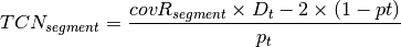
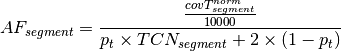
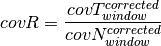
represents the observed tumor coverage of a segment. The factor \frac{1}{10000} is introduced to get from the initial 10 kb window coverage to a per base pair coverage. The 
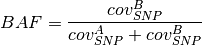
BAF value of a segment can be calculated as follows.

\label{eq:BAF}

where covT_{segment}^B 
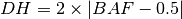
is the observed tumor coverage of a segment. The BAF value can now be used to calculate the DH of a segment according to [eq:DH]. Finally the allele-specific copy numbers are estimated.

\begin{aligned}
TCN_{segment}^B     & =  \frac{1}{2} \times TCN_{segment}  \times (1- DH_{segment}) \\
TCN_{segment}^A     & =  TCN_{segment} - TCN_{segment}^B \label{eq:TCNa}
\end{aligned}

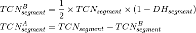
Purity and ploidy estimation

To obtain actual copy numbers for each segment ploidy and tumor cell content of the tumor sample have to be inferred from the data. Information about the allelic state of a segment is combined with TCN, DH and allele-specific copy numbers calculations. The combination of ploidy and tumor cell content that can explain the observed data the best is to be found. Possible ploidies in the range from 1 to 6.5 in steps of 0.1 and possible tumor cell content from 30% to 100% in steps of 1% are tested. The evaluation is done based on the distance of all segments from their next plausible copy number state. Imbalanced segments are fitted to a positive integer value.

\begin{aligned}
distance_{tcn\_imbalanced} & = abs( TCN_{segment} - round(TCN_{segment}) )
\end{aligned}

In addition the allele specific copy number is estimated according to equation [eq:TCNb] and [eq:TCNa]. For each allele a distance is defined accordingly:

\begin{aligned}
distance_{tcn\_a\_imbalanced} & = abs( TCN^{A}_{segment} - round(TCN^{A}_{segment}) ) \\
distance_{tcn\_b\_imbalanced} & = abs( TCN^{B}_{segment} - round(TCN^{B}_{segment}) )
\end{aligned}

The total distance as quality measure of a fit is defined as the sum of the distances.

\label{eq:totalDistImbalanced}
distance_{segment\_imbalanced}= distance_{tcn\_imbalanced} + distance_{tcn\_a\_imbalanced} +distance_{tcn\_b\_imbalanced}

Balanced segments can only be fitted to even total copy numbers. The distance is defined as follows:

\begin{aligned}
\label{eq:distTCNBalanced}
distance_{tcn\_balanced} = \frac{TCN_{segment}}{2} - floor(\frac{TCN_{segment} }{2})\\
?identical to\\
distance_{tcn\_balanced} = abs(\frac{TCN_{segment}}{2} - round(\frac{TCN_{segment} }{2}) ) \times 2
\end{aligned}

As both alleles are expected to be present in equal numbers the allele specific copy number as well as the total distance can be derived.

\begin{aligned}
distance_{tcn\_a\_balanced} & = distance_{tcn\_b\_balanced}  = \frac {distance_{tcn\_balanced} } {2}  \\
distance_{segment\_balanced} & =  distance_{tcn\_balanced} + distance_{tcn\_a\_balanced} + distance_{tcn\_b\_balanced} \\
& = 2 \times distance_{tcn\_balanced}
\end{aligned}

For each ploidy and tumor cell content combination a mean distance is defined by using the segment length as weights:

meanDist(p_t, P_t) = \frac{\sum_{1:N_{segments}}^{i}(distance_{segment_i} * length_{segment_i})} {\sum_{1:N_{segments}}^{i}{length_{segment_i}}}

All segments on diploid chromosomes that exceed a pre-set length and contain a sufficient amount of heterozygous SNP positions are used for the estimation. The smaller the distance the more likely a combination is chosen as final solution. Combinations of ploidy and tumor cell content that lead to negative copy numbers or exceed the DH limits are excluded as solution and used to set a minimum limit.

Final output

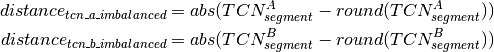
Once the optimal ploidy and tumor cell content combinations are found the TCN and allele-specific CN will be estimated for all segments in the genome and classified (gain, loss, copy-neutral LOH, loss LOH, gain LOH, sub). If a segments TCN is further than 0.3 away from an integer value it is assumed to originate from subpopulations in the tumor sample that lead to gains or losses in part of the tumor cell population.